
- Home
- Google Certification
- Professional-Machine-Learning-Engineer Exam
- Google.Professional-Machine-Learning-Engineer.v2025-05-29.q260 Practice Test

Question 6
You developed a custom model by using Vertex Al to forecast the sales of your company s products based on historical transactional data You anticipate changes in the feature distributions and the correlations between the features in the near future You also expect to receive a large volume of prediction requests You plan to use Vertex Al Model Monitoring for drift detection and you want to minimize the cost. What should you do?
Correct Answer: D
The best option for using Vertex AI Model Monitoring for drift detection and minimizing the cost is to use the features and the feature attributions for monitoring, and set a prediction-sampling-rate value that is closer to 0 than 1. This option allows you to leverage the power and flexibility of Google Cloud to detect feature drift in the input predict requests for custom models, and reduce the storage and computation costs of the model monitoring job. Vertex AI Model Monitoring is a service that can track and compare the results of multiple machine learning runs. Vertex AI Model Monitoring can monitor the model's prediction input data for feature skew and drift. Feature drift occurs when the feature data distribution in production changes over time. If the original training data is not available, you can enable drift detection to monitor your models for feature drift.
Vertex AI Model Monitoring uses TensorFlow Data Validation (TFDV) to calculate the distributions and distance scores for each feature, and compares them with a baseline distribution. The baseline distribution is the statistical distribution of the feature's values in the training data. If the training data is not available, the baseline distribution is calculated from the first 1000 prediction requests that the model receives. If the distance score for a feature exceeds an alerting threshold that you set, Vertex AI Model Monitoring sends you an email alert. However, if you use a custom model, you can also enable feature attribution monitoring, which can provide more insights into the feature drift. Feature attribution monitoring analyzes the feature attributions, which are the contributions of each feature to the prediction output. Feature attribution monitoring can help you identify the features that have the most impact on the model performance, and the features that have the most significant drift over time. Feature attribution monitoring can also help you understand the relationship between the features and the prediction output, and the correlation between the features1. The prediction-sampling-rate is a parameter that determines the percentage of prediction requests that are logged and analyzed by the model monitoring job. Using a lower prediction-sampling-rate can reduce the storage and computation costs of the model monitoring job, but also the quality and validity of the data. Using a lower prediction-sampling-rate can introduce sampling bias and noise into the data, and make the model monitoring job miss some important features or patterns of the data. However, using a higher prediction-sampling-rate can increase the storage and computation costs of the model monitoring job, and also the amount of data that needs to be processed and analyzed. Therefore, there is a trade-off between the prediction-sampling-rate and the cost and accuracy of the model monitoring job, and the optimal prediction-sampling-rate depends on the business objective and the data characteristics2. By using the features and the feature attributions for monitoring, and setting a prediction-sampling-rate value that is closer to 0 than 1, you can use Vertex AI Model Monitoring for drift detection and minimize the cost.
The other options are not as good as option D, for the following reasons:
* Option A: Using the features for monitoring and setting a monitoring-frequency value that is higher than the default would not enable feature attribution monitoring, and could increase the cost of the model monitoring job. The monitoring-frequency is a parameter that determines how often the model monitoring job analyzes the logged prediction requests and calculates the distributions and distance scores for each feature. Using a higher monitoring-frequency can increase the frequency and timeliness of the model monitoring job, but also the computation costs of the model monitoring job. Moreover, using the features for monitoring would not enable feature attribution monitoring, which can provide more insights into the feature drift and the model performance1.
* Option B: Using the features for monitoring and setting a prediction-sampling-rate value that is closer to
1 than 0 would not enable feature attribution monitoring, and could increase the cost of the model monitoring job. The prediction-sampling-rate is a parameter that determines the percentage of prediction requests that are logged and analyzed by the model monitoring job. Using a higher prediction-sampling-rate can increase the quality and validity of the data, but also the storage and computation costs of the model monitoring job. Moreover, using the features for monitoring would not enable feature attribution monitoring, which can provide more insights into the feature drift and the model performance12.
* Option C: Using the features and the feature attributions for monitoring and setting a monitoring-frequency value that is lower than the default would enable feature attribution monitoring, but could reduce the frequency and timeliness of the model monitoring job. The monitoring-frequency is a parameter that determines how often the model monitoring job analyzes the logged prediction requests and calculates the distributions and distance scores for each feature. Using a lower
* monitoring-frequency can reduce the computation costs of the model monitoring job, but also the frequency and timeliness of the model monitoring job. This can make the model monitoring job less responsive and effective in detecting and alerting the feature drift1.
References:
* Preparing for Google Cloud Certification: Machine Learning Engineer, Course 3: Production ML Systems, Week 4: Evaluation
* Google Cloud Professional Machine Learning Engineer Exam Guide, Section 3: Scaling ML models in production, 3.3 Monitoring ML models in production
* Official Google Cloud Certified Professional Machine Learning Engineer Study Guide, Chapter 6:
Production ML Systems, Section 6.3: Monitoring ML Models
* Using Model Monitoring
* Understanding the score threshold slider
Vertex AI Model Monitoring uses TensorFlow Data Validation (TFDV) to calculate the distributions and distance scores for each feature, and compares them with a baseline distribution. The baseline distribution is the statistical distribution of the feature's values in the training data. If the training data is not available, the baseline distribution is calculated from the first 1000 prediction requests that the model receives. If the distance score for a feature exceeds an alerting threshold that you set, Vertex AI Model Monitoring sends you an email alert. However, if you use a custom model, you can also enable feature attribution monitoring, which can provide more insights into the feature drift. Feature attribution monitoring analyzes the feature attributions, which are the contributions of each feature to the prediction output. Feature attribution monitoring can help you identify the features that have the most impact on the model performance, and the features that have the most significant drift over time. Feature attribution monitoring can also help you understand the relationship between the features and the prediction output, and the correlation between the features1. The prediction-sampling-rate is a parameter that determines the percentage of prediction requests that are logged and analyzed by the model monitoring job. Using a lower prediction-sampling-rate can reduce the storage and computation costs of the model monitoring job, but also the quality and validity of the data. Using a lower prediction-sampling-rate can introduce sampling bias and noise into the data, and make the model monitoring job miss some important features or patterns of the data. However, using a higher prediction-sampling-rate can increase the storage and computation costs of the model monitoring job, and also the amount of data that needs to be processed and analyzed. Therefore, there is a trade-off between the prediction-sampling-rate and the cost and accuracy of the model monitoring job, and the optimal prediction-sampling-rate depends on the business objective and the data characteristics2. By using the features and the feature attributions for monitoring, and setting a prediction-sampling-rate value that is closer to 0 than 1, you can use Vertex AI Model Monitoring for drift detection and minimize the cost.
The other options are not as good as option D, for the following reasons:
* Option A: Using the features for monitoring and setting a monitoring-frequency value that is higher than the default would not enable feature attribution monitoring, and could increase the cost of the model monitoring job. The monitoring-frequency is a parameter that determines how often the model monitoring job analyzes the logged prediction requests and calculates the distributions and distance scores for each feature. Using a higher monitoring-frequency can increase the frequency and timeliness of the model monitoring job, but also the computation costs of the model monitoring job. Moreover, using the features for monitoring would not enable feature attribution monitoring, which can provide more insights into the feature drift and the model performance1.
* Option B: Using the features for monitoring and setting a prediction-sampling-rate value that is closer to
1 than 0 would not enable feature attribution monitoring, and could increase the cost of the model monitoring job. The prediction-sampling-rate is a parameter that determines the percentage of prediction requests that are logged and analyzed by the model monitoring job. Using a higher prediction-sampling-rate can increase the quality and validity of the data, but also the storage and computation costs of the model monitoring job. Moreover, using the features for monitoring would not enable feature attribution monitoring, which can provide more insights into the feature drift and the model performance12.
* Option C: Using the features and the feature attributions for monitoring and setting a monitoring-frequency value that is lower than the default would enable feature attribution monitoring, but could reduce the frequency and timeliness of the model monitoring job. The monitoring-frequency is a parameter that determines how often the model monitoring job analyzes the logged prediction requests and calculates the distributions and distance scores for each feature. Using a lower
* monitoring-frequency can reduce the computation costs of the model monitoring job, but also the frequency and timeliness of the model monitoring job. This can make the model monitoring job less responsive and effective in detecting and alerting the feature drift1.
References:
* Preparing for Google Cloud Certification: Machine Learning Engineer, Course 3: Production ML Systems, Week 4: Evaluation
* Google Cloud Professional Machine Learning Engineer Exam Guide, Section 3: Scaling ML models in production, 3.3 Monitoring ML models in production
* Official Google Cloud Certified Professional Machine Learning Engineer Study Guide, Chapter 6:
Production ML Systems, Section 6.3: Monitoring ML Models
* Using Model Monitoring
* Understanding the score threshold slider
Question 7
You deployed an ML model into production a year ago. Every month, you collect all raw requests that were sent to your model prediction service during the previous month. You send a subset of these requests to a human labeling service to evaluate your model's performance. After a year, you notice that your model's performance sometimes degrades significantly after a month, while other times it takes several months to notice any decrease in performance. The labeling service is costly, but you also need to avoid large performance degradations. You want to determine how often you should retrain your model to maintain a high level of performance while minimizing cost. What should you do?
Correct Answer: D
The best option for determining how often to retrain your model to maintain a high level of performance while minimizing cost is to run training-serving skew detection batch jobs every few days. Training-serving skew refers to the discrepancy between the distributions of the features in the training dataset and the serving data. This can cause the model to perform poorly on the new data, as it is not representative of the data that the model was trained on. By running training-serving skew detection batch jobs, you can monitor the changes in the feature distributions over time, and identify when the skew becomes significant enough to affect the model performance. If skew is detected, you can send the most recent serving data to the labeling service, and use the labeled data to retrain your model. This option has the following benefits:
* It allows you to retrain your model only when necessary, based on the actual data changes, rather than on a fixed schedule or a heuristic. This can save you the cost of the labeling service and the retraining process, and also avoid overfitting or underfitting your model.
* It leverages the existing tools and frameworks for training-serving skew detection, such as TensorFlow Data Validation (TFDV) and Vertex Data Labeling. TFDV is a library that can compute and visualize descriptive statistics for your datasets, and compare the statistics across different datasets. Vertex Data Labeling is a service that can label your data with high quality and low latency, using either human labelers or automated labelers.
* It integrates well with the MLOps practices, such as continuous integration and continuous delivery (CI
/CD), which can automate the workflow of running the skew detection jobs, sending the data to the labeling service, retraining the model, and deploying the new model version.
The other options are less optimal for the following reasons:
* Option A: Training an anomaly detection model on the training dataset, and running all incoming requests through this model, introduces additional complexity and overhead. This option requires building and maintaining a separate model for anomaly detection, which can be challenging and time- consuming. Moreover, this option requires running the anomaly detection model on every request, which can increase the latency and resource consumption of the prediction service. Additionally, this option may not capture the subtle changes in the feature distributions that can affect the model performance, as anomalies are usually defined as rare or extreme events.
* Option B: Identifying temporal patterns in your model's performance over the previous year, and creating a schedule for sending serving data to the labeling service for the next year, introduces additional assumptions and risks. This option requires analyzing the historical data and model performance, and finding the patterns that can explain the variations in the model performance over time. However, this can be difficult and unreliable, as the patterns may not be consistent or predictable, and may depend on various factors that are not captured by the data. Moreover, this option requires creating a schedule based on the past patterns, which may not reflect the future changes in the data or the environment. This can lead to either sending too much or too little data to the labeling service, resulting in either wasted cost or degraded performance.
* Option C: Comparing the cost of the labeling service with the lost revenue due to model performance degradation over the past year, and adjusting the frequency of model retraining accordingly, introduces additional challenges and trade-offs. This option requires estimating the cost of the labeling service and the lost revenue due to model performance degradation, which can be difficult and inaccurate, as they may depend on various factors that are not easily quantifiable or measurable. Moreover, this option requires finding the optimal balance between the cost and the performance, which can be subjective and variable, as different stakeholders may have different preferences and expectations. Furthermore, this option may not account for the potential impact of the model performance degradation on other aspects of the business, such as customer satisfaction, retention, or loyalty.
* It allows you to retrain your model only when necessary, based on the actual data changes, rather than on a fixed schedule or a heuristic. This can save you the cost of the labeling service and the retraining process, and also avoid overfitting or underfitting your model.
* It leverages the existing tools and frameworks for training-serving skew detection, such as TensorFlow Data Validation (TFDV) and Vertex Data Labeling. TFDV is a library that can compute and visualize descriptive statistics for your datasets, and compare the statistics across different datasets. Vertex Data Labeling is a service that can label your data with high quality and low latency, using either human labelers or automated labelers.
* It integrates well with the MLOps practices, such as continuous integration and continuous delivery (CI
/CD), which can automate the workflow of running the skew detection jobs, sending the data to the labeling service, retraining the model, and deploying the new model version.
The other options are less optimal for the following reasons:
* Option A: Training an anomaly detection model on the training dataset, and running all incoming requests through this model, introduces additional complexity and overhead. This option requires building and maintaining a separate model for anomaly detection, which can be challenging and time- consuming. Moreover, this option requires running the anomaly detection model on every request, which can increase the latency and resource consumption of the prediction service. Additionally, this option may not capture the subtle changes in the feature distributions that can affect the model performance, as anomalies are usually defined as rare or extreme events.
* Option B: Identifying temporal patterns in your model's performance over the previous year, and creating a schedule for sending serving data to the labeling service for the next year, introduces additional assumptions and risks. This option requires analyzing the historical data and model performance, and finding the patterns that can explain the variations in the model performance over time. However, this can be difficult and unreliable, as the patterns may not be consistent or predictable, and may depend on various factors that are not captured by the data. Moreover, this option requires creating a schedule based on the past patterns, which may not reflect the future changes in the data or the environment. This can lead to either sending too much or too little data to the labeling service, resulting in either wasted cost or degraded performance.
* Option C: Comparing the cost of the labeling service with the lost revenue due to model performance degradation over the past year, and adjusting the frequency of model retraining accordingly, introduces additional challenges and trade-offs. This option requires estimating the cost of the labeling service and the lost revenue due to model performance degradation, which can be difficult and inaccurate, as they may depend on various factors that are not easily quantifiable or measurable. Moreover, this option requires finding the optimal balance between the cost and the performance, which can be subjective and variable, as different stakeholders may have different preferences and expectations. Furthermore, this option may not account for the potential impact of the model performance degradation on other aspects of the business, such as customer satisfaction, retention, or loyalty.
Question 8
You work for a retail company. You have a managed tabular dataset in Vertex Al that contains sales data from three different stores. The dataset includes several features such as store name and sale timestamp. You want to use the data to train a model that makes sales predictions for a new store that will open soon You need to split the data between the training, validation, and test sets What approach should you use to split the data?
Correct Answer: B
The best option for splitting the data between the training, validation, and test sets, using a managed tabular dataset in Vertex AI that contains sales data from three different stores, is to use Vertex AI default data split.
This option allows you to leverage the power and simplicity of Vertex AI to automatically and randomly split your data into the three sets by percentage. Vertex AI is a unified platform for building and deploying machine learning solutions on Google Cloud. Vertex AI can support various types of models, such as linear regression, logistic regression, k-means clustering, matrix factorization, and deep neural networks. Vertex AI can also provide various tools and services for data analysis, model development, model deployment, model monitoring, and model governance. A default data split is a data split method that is provided by Vertex AI, and does not require any user input or configuration. A default data split can help you split your data into the training, validation, and test sets by using a random sampling method, and assign a fixed percentage of the data to each set. A default data split can help you simplify the data split process, and works well in most cases.
A training set is a subset of the data that is used to train the model, and adjust the model parameters. A training set can help you learn the relationship between the input features and the target variable, and optimize the model performance. A validation set is a subset of the data that is used to validate the model, and tune the model hyperparameters. A validation set can help you evaluate the model performance on unseen data, and avoid overfitting or underfitting. A test set is a subset of the data that is used to test the model, and provide the final evaluation metrics. A test set can help you assess the model performance on new data, and measure the generalization ability of the model. By using Vertex AI default data split, you can split your data into the training, validation, and test sets by using a random sampling method, and assign the following percentages of the data to each set1:

The other options are not as good as option B, for the following reasons:
* Option A: Using Vertex AI manual split, using the store name feature to assign one store for each set would not allow you to split your data into representative and balanced sets, and could cause errors or poor performance. A manual split is a data split method that allows you to control how your data is split into sets, by using the ml_use label or the data filter expression. A manual split can help you customize the data split logic, and handle complex or non-standard data formats. A store name feature is a feature that indicates the name of the store where the sales data was collected. A store name feature can help you identify the source of the data, and group the data by store. However, using Vertex AI manual split, using the store name feature to assign one store for each set would not allow you to split your data into representative and balanced sets, and could cause errors or poor performance. You would need to write code, create and configure the ml_use label or the data filter expression, and assign one store for each set. Moreover, this option would not ensure that the data in each set has the same distribution and characteristics as the data in the whole dataset, which could prevent you from learning the general pattern of the data, and cause bias or variance in the model2.
* Option C: Using Vertex AI chronological split and specifying the sales timestamp feature as the time variable would not allow you to split your data into representative and balanced sets, and could cause errors or poor performance. A chronological split is a data split method that allows you to split your data into sets based on the order of the data. A chronological split can help you preserve the temporal dependency and sequence of the data, and avoid data leakage. A sales timestamp feature is a feature that indicates the date and time when the sales data was collected. A sales timestamp feature can help you track the changes and trends of the data over time, and capture the seasonality and cyclicality of the data. However, using Vertex AI chronological split and specifying the sales timestamp feature as the time variable would not allow you to split your data into representative and balanced sets, and could cause errors or poor performance. You would need to write code, create and configure the time variable, and split the data by the order of the time variable. Moreover, this option would not ensure that the data in each set has the same distribution and characteristics as the data in the whole dataset, which could prevent you from learning the general pattern of the data, and cause bias or variance in the model3.
* Option D: Using Vertex AI random split, assigning 70% of the rows to the training set, 10% to the validation set, and 20% to the test set would not allow you to use the default data split method that is provided by Vertex AI, and could increase the complexity and cost of the data split process. A random split is a data split method that allows you to split your data into sets by using a random sampling method, and assign a custom percentage of the data to each set. A random split can help you split your data into representative and balanced sets, and avoid data leakage. However, using Vertex AI random split, assigning 70% of the rows to the training set, 10% to the validation set, and 20% to the test set would not allow you to use the default data split method that is provided by Vertex AI, and could increase the complexity and cost of the data split process. You would need to write code, create and
* configure the random split method, and assign the custom percentages to each set. Moreover, this option would not use the default data split method that is provided by Vertex AI, which can simplify the data split process, and works well in most cases1.
References:
* About data splits for AutoML models | Vertex AI | Google Cloud
* Manual split for unstructured data
* Mathematical split
This option allows you to leverage the power and simplicity of Vertex AI to automatically and randomly split your data into the three sets by percentage. Vertex AI is a unified platform for building and deploying machine learning solutions on Google Cloud. Vertex AI can support various types of models, such as linear regression, logistic regression, k-means clustering, matrix factorization, and deep neural networks. Vertex AI can also provide various tools and services for data analysis, model development, model deployment, model monitoring, and model governance. A default data split is a data split method that is provided by Vertex AI, and does not require any user input or configuration. A default data split can help you split your data into the training, validation, and test sets by using a random sampling method, and assign a fixed percentage of the data to each set. A default data split can help you simplify the data split process, and works well in most cases.
A training set is a subset of the data that is used to train the model, and adjust the model parameters. A training set can help you learn the relationship between the input features and the target variable, and optimize the model performance. A validation set is a subset of the data that is used to validate the model, and tune the model hyperparameters. A validation set can help you evaluate the model performance on unseen data, and avoid overfitting or underfitting. A test set is a subset of the data that is used to test the model, and provide the final evaluation metrics. A test set can help you assess the model performance on new data, and measure the generalization ability of the model. By using Vertex AI default data split, you can split your data into the training, validation, and test sets by using a random sampling method, and assign the following percentages of the data to each set1:
The other options are not as good as option B, for the following reasons:
* Option A: Using Vertex AI manual split, using the store name feature to assign one store for each set would not allow you to split your data into representative and balanced sets, and could cause errors or poor performance. A manual split is a data split method that allows you to control how your data is split into sets, by using the ml_use label or the data filter expression. A manual split can help you customize the data split logic, and handle complex or non-standard data formats. A store name feature is a feature that indicates the name of the store where the sales data was collected. A store name feature can help you identify the source of the data, and group the data by store. However, using Vertex AI manual split, using the store name feature to assign one store for each set would not allow you to split your data into representative and balanced sets, and could cause errors or poor performance. You would need to write code, create and configure the ml_use label or the data filter expression, and assign one store for each set. Moreover, this option would not ensure that the data in each set has the same distribution and characteristics as the data in the whole dataset, which could prevent you from learning the general pattern of the data, and cause bias or variance in the model2.
* Option C: Using Vertex AI chronological split and specifying the sales timestamp feature as the time variable would not allow you to split your data into representative and balanced sets, and could cause errors or poor performance. A chronological split is a data split method that allows you to split your data into sets based on the order of the data. A chronological split can help you preserve the temporal dependency and sequence of the data, and avoid data leakage. A sales timestamp feature is a feature that indicates the date and time when the sales data was collected. A sales timestamp feature can help you track the changes and trends of the data over time, and capture the seasonality and cyclicality of the data. However, using Vertex AI chronological split and specifying the sales timestamp feature as the time variable would not allow you to split your data into representative and balanced sets, and could cause errors or poor performance. You would need to write code, create and configure the time variable, and split the data by the order of the time variable. Moreover, this option would not ensure that the data in each set has the same distribution and characteristics as the data in the whole dataset, which could prevent you from learning the general pattern of the data, and cause bias or variance in the model3.
* Option D: Using Vertex AI random split, assigning 70% of the rows to the training set, 10% to the validation set, and 20% to the test set would not allow you to use the default data split method that is provided by Vertex AI, and could increase the complexity and cost of the data split process. A random split is a data split method that allows you to split your data into sets by using a random sampling method, and assign a custom percentage of the data to each set. A random split can help you split your data into representative and balanced sets, and avoid data leakage. However, using Vertex AI random split, assigning 70% of the rows to the training set, 10% to the validation set, and 20% to the test set would not allow you to use the default data split method that is provided by Vertex AI, and could increase the complexity and cost of the data split process. You would need to write code, create and
* configure the random split method, and assign the custom percentages to each set. Moreover, this option would not use the default data split method that is provided by Vertex AI, which can simplify the data split process, and works well in most cases1.
References:
* About data splits for AutoML models | Vertex AI | Google Cloud
* Manual split for unstructured data
* Mathematical split
Question 9
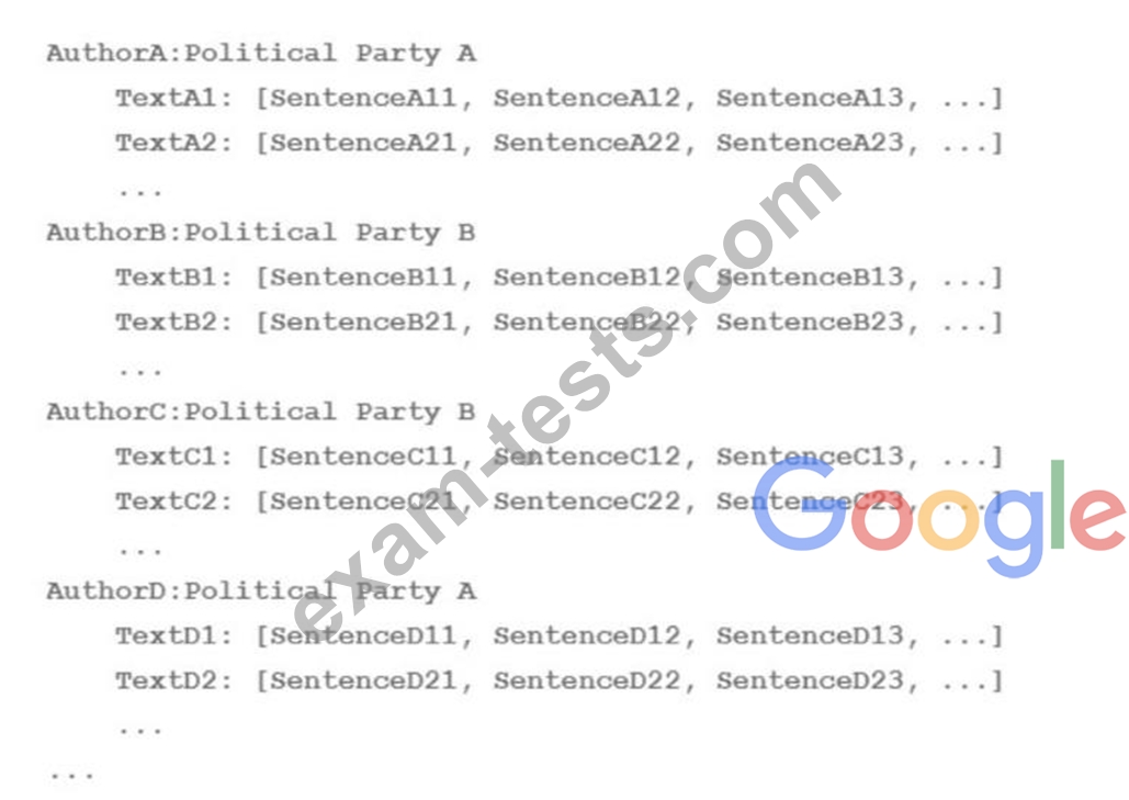
Your team is working on an NLP research project to predict political affiliation of authors based on articles they have written. You have a large training dataset that is structured like this:
A)
B)

C)

D)

A)
B)
C)
D)
Correct Answer: B
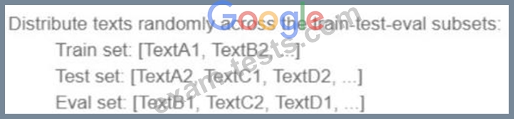
If we just put inside the Training set , Validation set and Test set , randomly Text, Paragraph or sentences the model will have the ability to learn specific qualities about The Author's use of language beyond just his own articles. Therefore the model will mixed up different opinions. Rather if we divided things up a the author level, so that given authors were only on the training data, or only in the test data or only in the validation data. The model will find more difficult to get a high accuracy on the test validation (What is correct and have more sense!). Because it will need to really focus in author by author articles rather than get a single political affiliation based on a bunch of mixed articles from different authors. https://developers.google.com/machine-learning/crash-course/18th-century-literature For example, suppose you are training a model with purchase data from a number of stores. You know, however, that the model will be used primarily to make predictions for stores that are not in the training data. To ensure that the model can generalize to unseen stores, you should segregate your data sets by stores. In other words, your test set should include only stores different from the evaluation set, and the evaluation set should include only stores different from the training set. https://cloud.google.com/automl-tables/docs/prepare#ml-use
Question 10
You are going to train a DNN regression model with Keras APIs using this code:

How many trainable weights does your model have? (The arithmetic below is correct.)
How many trainable weights does your model have? (The arithmetic below is correct.)
Correct Answer: B
The number of trainable weights in a DNN regression model with Keras APIs can be calculated by multiplying the number of input units by the number of output units for each layer, and adding the number of bias units for each layer. The bias units are usually equal to the number of output units, except for the last layer, which does not have bias units if the activation function is softmax1. In this code, the model has three layers: a dense layer with 256 units and relu activation, a dropout layer with 0.25 rate, and a dense layer with
2 units and softmax activation. The input shape is 500. Therefore, the number of trainable weights is:
* For the first layer: 500 input units * 256 output units + 256 bias units = 128256
* For the second layer: The dropout layer does not have any trainable weights, as it only randomly sets some of the input units to zero to prevent overfitting2.
* For the third layer: 256 input units * 2 output units + 0 bias units = 512 The total number of trainable weights is 128256 + 512 = 161024. Therefore, the correct answer is B.
References:
* How to calculate the number of parameters for a Convolutional Neural Network?
* Dropout (keras.io)
2 units and softmax activation. The input shape is 500. Therefore, the number of trainable weights is:
* For the first layer: 500 input units * 256 output units + 256 bias units = 128256
* For the second layer: The dropout layer does not have any trainable weights, as it only randomly sets some of the input units to zero to prevent overfitting2.
* For the third layer: 256 input units * 2 output units + 0 bias units = 512 The total number of trainable weights is 128256 + 512 = 161024. Therefore, the correct answer is B.
References:
* How to calculate the number of parameters for a Convolutional Neural Network?
* Dropout (keras.io)
- Other Version
- 3767Google.Professional-Machine-Learning-Engineer.v2024-09-13.q242
- 2751Google.Professional-Machine-Learning-Engineer.v2023-12-28.q120
- 1253Google.Professional-Machine-Learning-Engineer.v2023-02-27.q25
- 2604Google.Professional-Machine-Learning-Engineer.v2022-08-07.q66
- 2227Google.Professional-Machine-Learning-Engineer.v2022-03-21.q70
- 62Google.Prepawayete.Professional-Machine-Learning-Engineer.v2021-09-13.by.murray.54q.pdf
- Latest Upload
- 448PaloAltoNetworks.NGFW-Engineer.v2026-05-01.q43
- 584Nokia.4A0-113.v2026-05-01.q69
- 613EC-COUNCIL.312-49v11.v2026-04-30.q214
- 595Microsoft.MB-820.v2026-04-30.q101
- 439Salesforce.MC-202.v2026-04-30.q57
- 480BICSI.INSTC_V8.v2026-04-29.q53
- 581NMLS.MLO.v2026-04-28.q82
- 404NCARB.Project-Management.v2026-04-28.q27
- 759EMC.D-AV-DY-23.v2026-04-27.q184
- 1987ServiceNow.CSA.v2026-04-27.q483
[×]
Download PDF File
Enter your email address to download Google.Professional-Machine-Learning-Engineer.v2025-05-29.q260 Practice Test